Beat Effect in Sub-Nyquist Signals
Pablo Panitta
Introduction
This work aims to study the effect on signals whose frequencies are in the lower vicinity of the Nyquist frequency (called sub-Nyquist signals). We will begin by analysing the interaction between two analog signals and the effects that arise. Then, we will examine what happens in the digital domain regarding a signal's proximity to the Nyquist frequency. The implications for the graphical representation of signals and their impact on D/A conversion for playback will be addressed.
1. Sum of Two Analog Signals
Suppose we have two analog sinusoidal signals and add them together. What result will we see on an oscilloscope screen? If the difference between their frequencies is large (say, more than 10 times), we will see the higher-frequency sine wave superimposed on the lower-frequency one.
However, as this difference decreases, we will increasingly notice that the higher-frequency sine wave is "beaten" by the lower-frequency one.
In Figs. 1, 2, 3, and 4, the effects mentioned above can be observed.
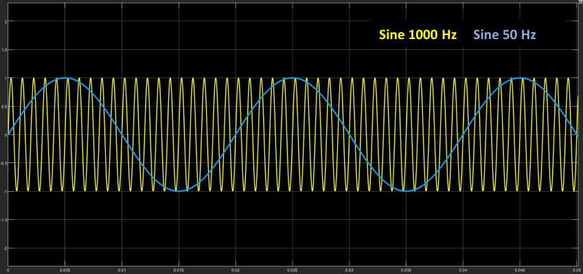
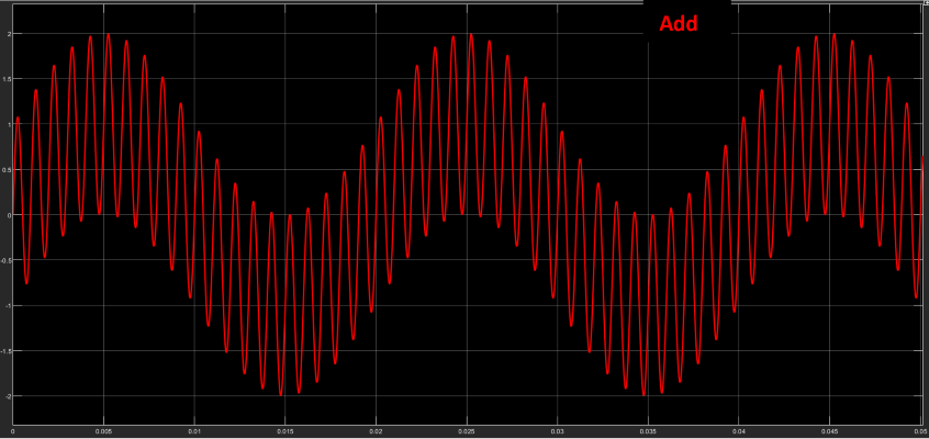
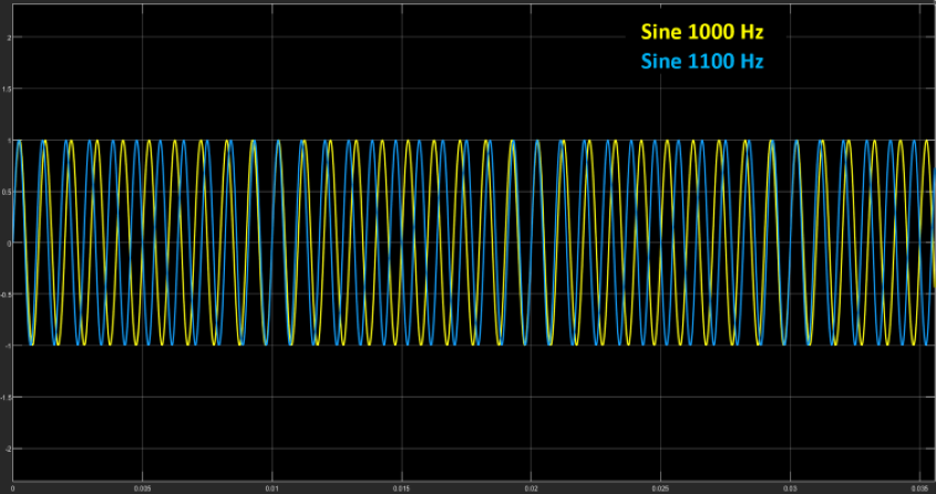
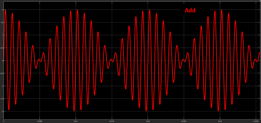
It is interesting to note the effect that phase has on the sum of signals in both combinations. While phase does not play a significant role when the frequency difference is large, it does when the frequencies are close, producing cancellations or reinforcements in the magnitude of the sum.
Note that the beat frequency is equal to the difference between the frequencies of both signals (in this case, 100Hz).[1][1]
In both cases, a spectral analysis will show only the two pure sinusoidal frequencies and nothing else.
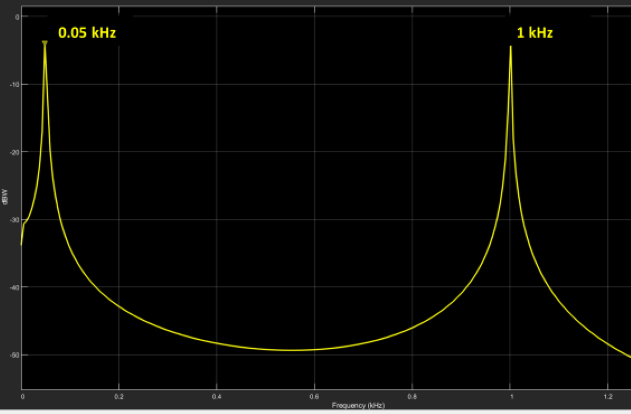
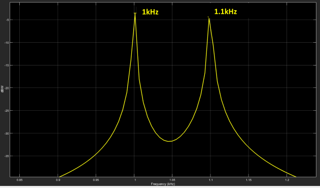
Fig 5. Spectrum of signals a) Scenario1, b) Scenario2
2. Beat in the Digital Domain
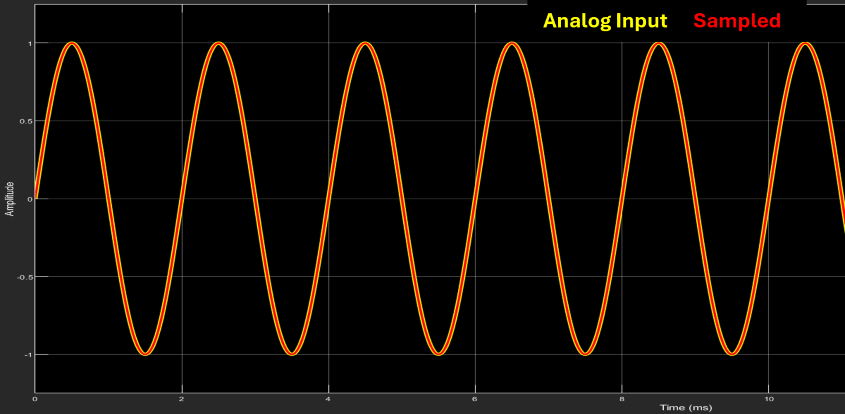
Now suppose we have an analog signal and proceed to sample it for digitization. For demonstration purposes, let’s take the following values:
- Signal frequency: 500 Hz
- Sampling frequency: 44.1kHz
In Fig 6, we can see that the sampled signal is perfectly overlaid on the analog signal, showing no amplitude deviations.
It is striking that if I wanted to reconstruct the signal by connecting the samples, I would not be obtaining the same original signal. As observed in Fig 12, if I apply the sampling process to a pure sinusoidal signal (A/D) and then, from those samples, reconstruct the signal (D/A) by connecting the samples, I would arrive at a sinusoidal signal but with a beat, which obviously is not the same as the original signal. But this would be a clear contradiction to the Nyquist theorem, which states that if I meet the condition of sampling at a rate higher than twice the maximum frequency present, I could reconstruct the original signal exactly.
Let’s repeat the process, but now with a frequency close to Nyquist, for example, a signal frequency of 20 kHz.
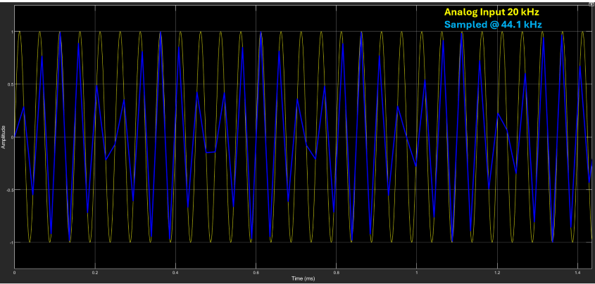
In Fig 7, we can clearly observe a beat effect on the 20kHz signal. This looks very similar to the effect described in the previous section with two analog frequencies. But if we are working with only one frequency here… how can this be happening?
Let’s try to understand what’s going on in this case. I have a 20kHz analog signal at the input, which, when sampled at a rate of 44.1kHz and then converted back to analog[2][2], appears as a 20kHz signal but with a beat at 4.1kHz. Everything suggests that, based on what we saw earlier, there should be another signal “modulating” the input to produce the modulated signal. Let’s confirm this with a spectrum analyzer.
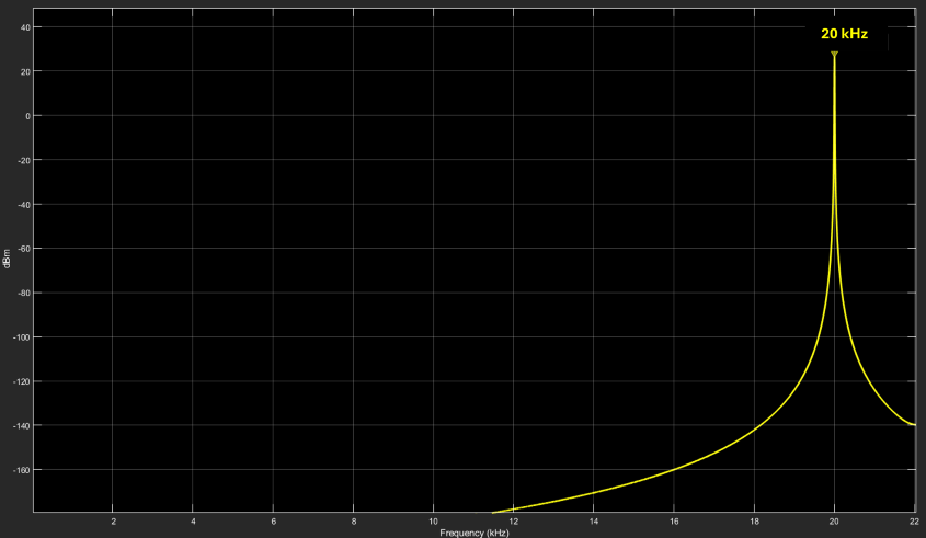
Undoubtedly, Fig 8 shows evidence of only one signal! This doesn’t seem to make much sense. There is only one signal present in the spectrum, yet in the time domain, it shows clear signs of amplitude modulation (beat) that could only occur if another signal were interacting.
So what’s going on?
3. Sample Distribution in a Signal
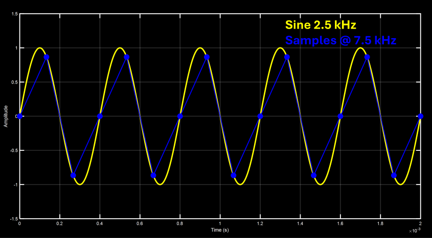
Suppose we sample a signal with frequency F at a sampling rate \( F_s = 3F \). What we would get is the presence of 3 samples per signal cycle, and furthermore, these occur at the same phase of the signal. In other words, a periodic pattern is created, as we can observe in Fig 9.
And if we did the same, but now with \( F_s = 5F \), there would be 5 samples per signal cycle, with the same characteristics as the previous signal, as can be seen in the following figure.
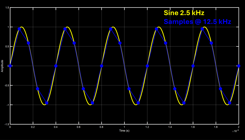
A particularity of the examples just mentioned is that the number of samples per signal cycle is invariant. This means that, for example, in \( F_s = 3F \), there will be 3, and only 3, samples in any signal cycle. I won’t find cycles with 2, 4, or any other number of samples. In other words, there is a relationship between F and \( F_s \) that we can represent with the following equation:
\[ {\large F = \frac{1}{n} \cdot F_s } \]Again, this means that every 1 cycle, I will have “n” (2, 3, 4, etc.) and only “n” samples. No more, no less.
We can generalize the formula and rewrite it as:
Here, m indicates the number of cycles in which I will find a number of n samples. For example, if the ratio were \( \large\frac{2}{5} \), it would mean that in 2 signal cycles, I will find exactly 5 samples.[3][3]
But there is another characteristic that has a very important consequence: n samples occur at the same phases of the signal every m cycles. Following the previous example, the samples will fall at the same phase of the signal every 2 cycles.
But where are we going with this? What does it have to do with what I see on the screen? A little more patience, and we’re getting closer.
4. Cyclic Patterns
Now let’s add one last parameter to the formula, called ε, so that it results as shown in the following equation:
\[ {\large F = \frac{m}{n} \cdot F_s - {\Large \varepsilon}} \]
What does this modification achieve? It cancels the fixed positioning characteristic of the samples within the signal cycle. Although there will still be n samples every m cycles, their location within the signal will vary across cycles.
And will the samples ever fall at the same phase of the wave again? In other words, will there be a frequency at which the cycle repeats? The answer is yes, and that is precisely the value of ε.
Let’s look at the graphs of some examples:
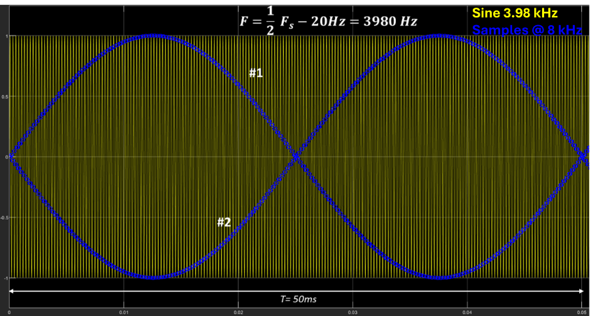
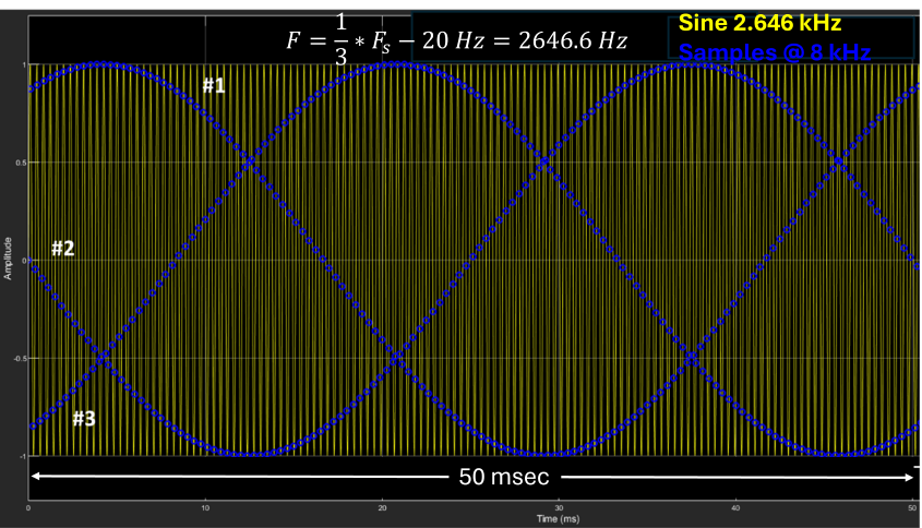
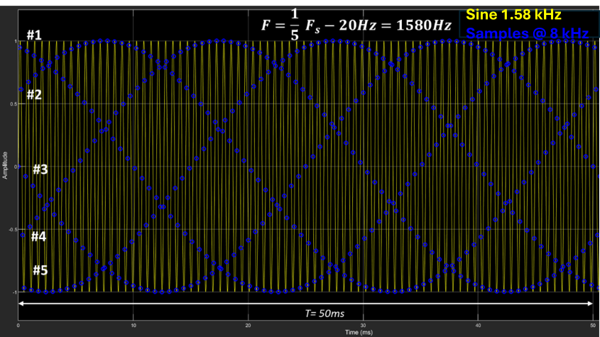
In Fig 11, we can observe the distribution of samples “forming” sinusoidal waves whose number corresponds to the value of the factor “n” and with a frequency of value ε.
In other words, in the formula \( F = {\large \frac{F_s}{2}} - 20 \), 2 waves will be formed; in \( F = {\large \frac{F_s}{3}} - 20 \), 3 waves; and in \( F = {\large \frac{F_s}{5}} - 20 \), 5 interlaced waves. All of them have a frequency of 20 Hz (as is the value of ε).
Note that these waves are the product of a graphical distribution of the signal’s samples, and all have a frequency of ε. This means that ε is the frequency at which the samples occur again at the same phase of the signal. It is easy to see that if ε=0, the variation frequency is 0, and therefore, the samples always occur at the same phase of the signal.
5. The Reconstruction Process

The explanation lies in how the reconstruction of the analog signal from its samples is performed. The interpolation process consists of reconstructing the signal value between samples, and this is not achieved by simply “connecting” the samples graphically. There are various ways to “connect” (interpolate) the samples graphically. For example, one could be to do it linearly (straight line), through an N-order polynomial (curve), or some other type.[4][4][5][5] But those methods do not reconstruct the original signal exactly.
The theoretical method to fully recover an analog signal (i.e., without loss) is through a convolution process between the samples and the SINC function. It is entirely beyond the scope of this work to explain the reconstruction (interpolation) process in detail, but we can think of it as follows: If I wanted to recover a frequency-limited signal (that meets Nyquist requirements), I could filter it with a low-pass filter to keep the frequency band below \( \frac{F_s}{2} \) and reject all spectral components above it. In Fig 13, we can see the process.
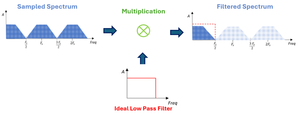
The mechanism of this filtering process, but viewed from the time domain (always remember the frequency-time duality), would mean a convolution between each of the samples and the SINC function, which is the time-domain representation of an ideal low-pass response.
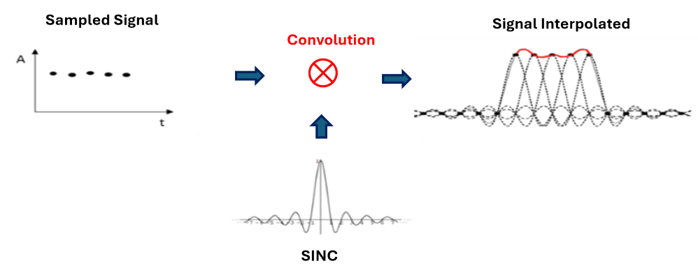
In theory, this process provides perfect reconstruction. But the problem lies in the impossibility of its implementation, as the SINC function extends from \(-\infty \) to \( +\infty \). Since this is not feasible for practical purposes, we must truncate it in time. This temporal truncation of the function will have an impact in the frequency domain, meaning that the low-pass filter response will no longer be ideal, and this will introduce “distortions” in the reconstruction of the analog signal. And it is precisely these errors that make the reconstructed signal more or less like the original.
In Appendix III, you will find a practical demonstration of the impact of the SINC length on the reconstruction process.
6. Is this Effect Real?
Having understood the reason for the “weird” shapes we see in the reconstruction of certain frequencies, it is worth asking whether this is a real effect or simply a visual effect. The answer is that this effect is as real as digital audio itself, so it is not only a visual perception but also an auditory one.
And verifying this is not difficult at all. You can simply create a session at some audible Nyquist frequency, generate a sinusoidal signal (or any periodic signal), and listen. For example, we can test with an Fs = 8000Hz and use a generator to create sinusoids at F = 3998 Hz and F=3999Hz.
Having reached this point (and hopefully understood the explanation) … what would you expect to hear? (4-second audios, be careful with the volume)
7. Impact on Digital Audio
But if this is the case… how is it not a complete disaster for everything we hear through digital audio?
Well, there are two important aspects to consider in the explained process:
1) While not exclusive, this is noticeable in periodic signals. The beat effect is evident when there are periodic repetitions of samples in the signal cycles (as explained in section 4).
2) The effect is extremely noticeable in frequencies very close to Nyquist and loses impact as we move away from it. If my Nyquist frequency is 22050 Hz, the effect begins to fade from 20 kHz downward. In other words, these are high frequencies for the average human hearing.[6][6]
In Fig 15, we can see the impact in relation to the analog frequency being sampled. As the frequency F moves away from \({\large\frac{F_s}{2}}\), the effect diminishes (the beat loses intensity).
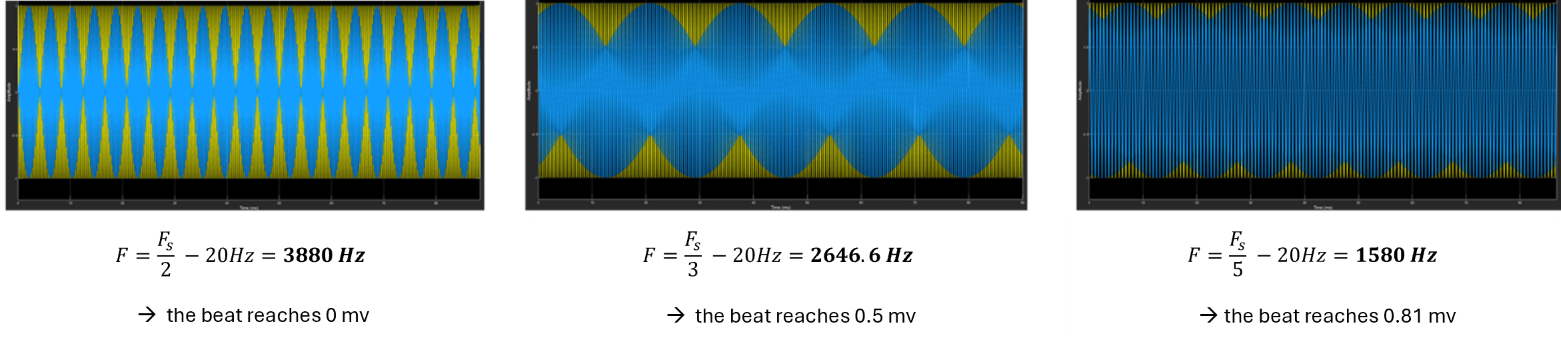
For these reasons, although it is curious to see it on DAW screens, this effect is not a problem for the purpose of digital audio.
Appendix I: Measurements
The following displays the measurements made at the output of a Universal Audio Apollo Twin sound card. The measurement instrument used was a Tektronix TBS 1052B, at different sampling and signal frequencies.
The measurement process consisted of generating sinusoids at different frequencies and measuring the analog audio output of the card. This is what the speakers will actually reproduce.
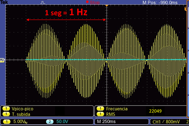
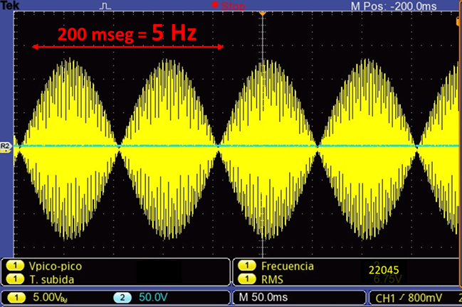
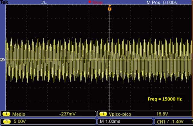
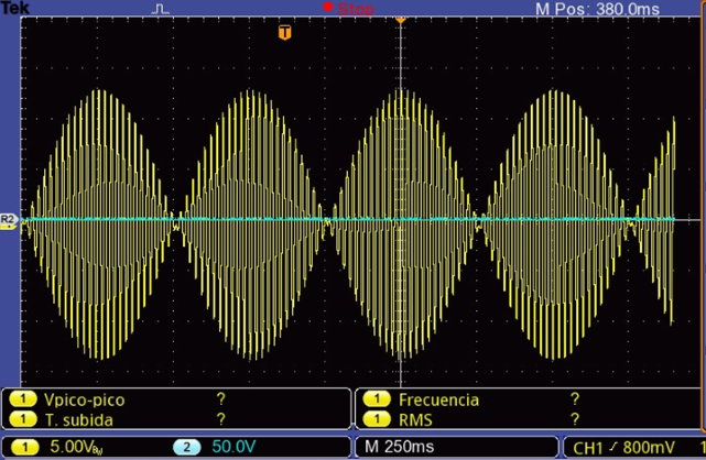
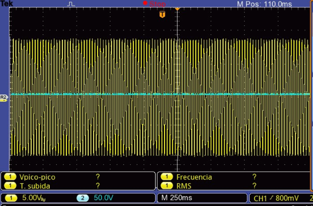
The impact can be observed for the same frequency at different sampling rates.
For 88200Hz, the impact is negligible, while for 44100Hz, it is noticeable.
Appendix II: Product of Two Analog Signals
According to the trigonometric identity:

We can create the same beat effect multiplying sinusoidal signals (instead of summing them), modifying the frequencies to satisfy this identity.[7][7] In our example of A=1000Hz and B=1100Hz, the new frequencies to achieve the same effect would be:
\( F_1 ={\large \frac{A + B}{2}} = 1050\,\text{Hz} \)
\( F_2 ={\large \frac{A - B}{2}} = 50\,\text{Hz} \)
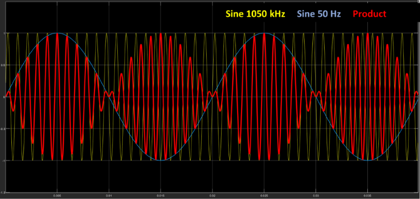
Fig 20. Beat effect through the product of signals
Note that the beat frequency remains 100Hz (as in the summing example), which is precisely twice the frequency of the modulator.
Appendix III: Interpolation Process of a Sampled Signal
It has been mentioned that, even when meeting the Nyquist criterion, we will have an imperfect reconstruction of the signal due to the limitation of having to truncate the SINC signal in the convolution process. We have also noted that this phenomenon is noticeable at frequencies close to Nyquist and that as we move away from it, the effect diminishes.
Below, three graphs are shown in which we can see how increasing the SINC duration significantly improves the reconstruction.[8][8]
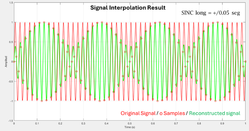
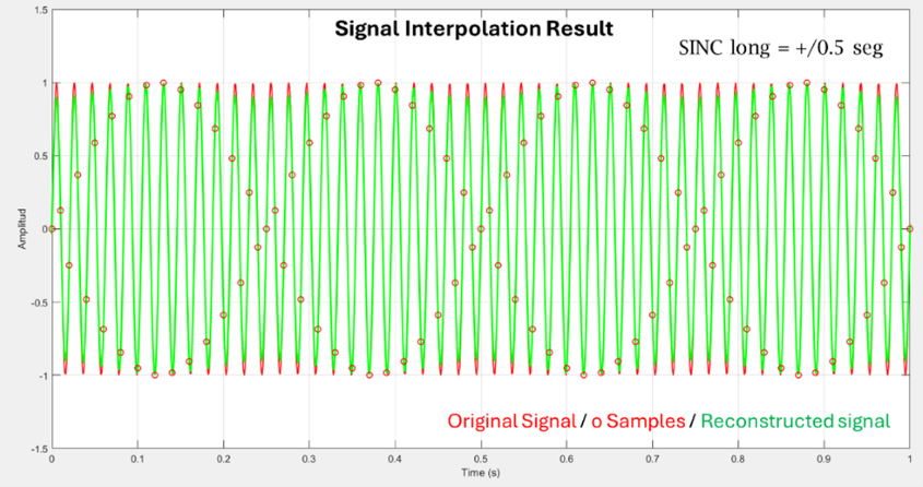
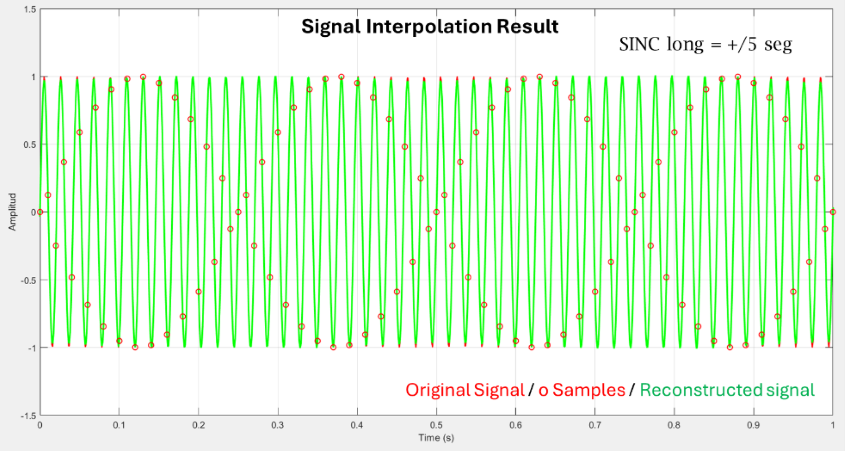
a) SINC_span=+/- 50 msec; b) SINC_span=+/- 500 msec; c) SINC_span=+/- 5 sec
The example presented corresponds to a \( F = 48\,\text{Hz} \) and \( F_s = 100\,\text{Hz} \). While these are not usable values in audio, they are perfectly valid for demonstrating the effect in question.
References
[1] The beat frequency is the difference between the two signals. However, the frequency of each of the interlaced waves is half, i.e., 50Hz in our case. This relationship will be different in the sub-Nyquist effect we will see in the following sections.
[2] Matlab’s interpolation method is linear, which is why we see straight lines connecting the samples.
[3] \(\large \frac{m}{n} \) ≤ 0.5 to avoid aliasing.
[4] There are several interpolation methods such as Lagrange (N-order), cubic splines (3rd order), Bezier splines, etc.
[5] Some software allows choosing the graphical interpolation mode (e.g., Ozone RX).
[6] Additionally, the beat is only perceived if its frequency is very low (no more than a few Hertz).
[7] This is the principle used in the amplitude modulation (AM) process. A low-frequency modulating signal (e.g., voice) modulates a much higher-frequency carrier for transmission.
[8] This is the result of a simulation, but it accurately reflects the stated theoretical concept. Obviously, this cannot be applied in the real world, as in DA converters, this duration is not adjustable.
Software and Hardware Used
The simulations carried out in this work were developed in MATLAB™.
Universal Audio Apollo Twin™ sound card.
Tektronix™ TBS 1052B measurement instrument.
Bibliography
- “Sub-Nyquist artefacts and sampling moiré effects” - Isaac Amidror, Ecole Polytechnique Fédérale de Lausanne (EPFL), Feb.Concurrent2015
- “Analyzing the Sampling-Induced Beat Frequency Effect” - Kerry Schutz – Mathwork, Oct 2021
- “Bandlimited Interpolation” – Julius O. Smith III - CCRMA – Stanford Univ, 2016 May
- “Modern Sampling: A Tutorial”. Jamie A.S. Angus – AES Vol 67, No 5, 2019 May
Author: Pablo Panitta / Soundins
Contact: pablopanitta@soundins.com.ar